Aquaveo & Water Resources Engineering News

Understanding Pass Through Cells

Starting with version 10.8, the Groundwater Modeling System (GMS) has the ability to handle pass through cells in MODFLOW-USG and MODFLOW-USG Transport projects. What are pass through cells? If you have a 3D UGrid with multiple layers, you can have middle layers with pinchouts or other features that cause that middle layer to not extend through the entire range of the other layers. For example, if you have a three-layer unstructured grid with a pinchout in layer two, then you will have an area where the cells of layer one and layer three are supposed to meet. This area where a middle layer is missing for some of the cells is where pass-through cells are needed.

In actuality, there is a thin cell between the layers. Because of this, in areas where a middle layer is missing a barrier would be formed when running MODFLOW-USG. If you don’t want a barrier in that area, then you will need to add a pass through cell to allow water to flow through the area. This means you need to have the Ibound be greater than zero or the water will not be able to pass through the middle layer and create a “no-flow zone.”

By switching between layers you can see which layers have a thickness of zero and which do not. To inactivate the cells with a thickness do the following:

  1. Open the MODFLOW Global/Basic Package dialog.
  2. Select the Set Pass Through… button.
  3. A message will appear explaining parameters used to determine pass through cells.
  4. In the Pass Through Thickness dialog, set the maximum cell thickness.
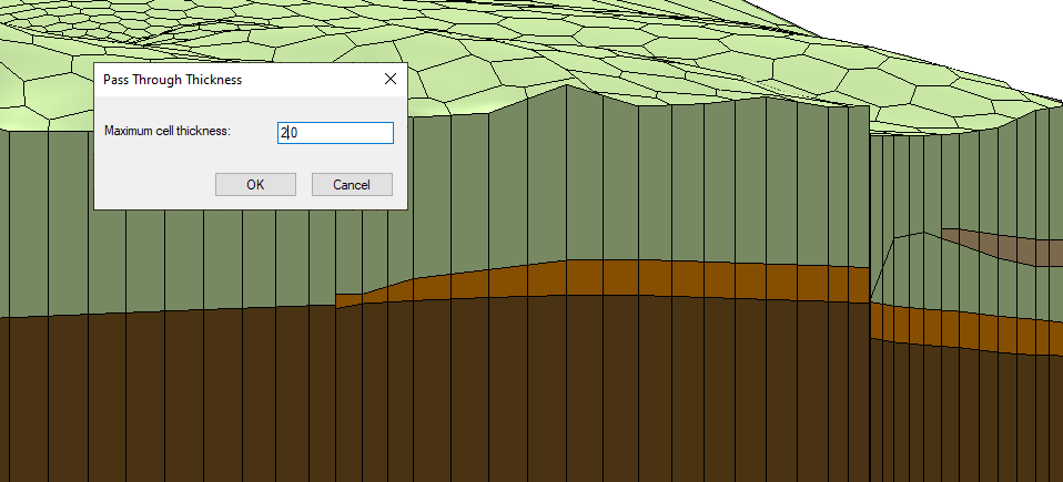
Example of setting pass through cells

After assigning the maximum cell thickness, cells that are below that thickness will be designated as pass through cells. The pass through cells will have an inactive IBOUND and will be ignored when making vertical connections in the DISU package.

Note that setting pass through cells requires a stacked grid.

Now that you know about pass through cells, make use of them in your MODFLOW-USG and MODFLOW-USG Transport projects in GMS today!
Blog tags: 

Tips for Long Term Precipitaiton Simulations

The Watershed Modeling System (WMS) has several options for modeling rainfall events, however many of them are built to model only single rainfall events. If you are looking to create long term simulations that include precipitation, the Gridded Surface Subsurface Hydrologic Analysis (GSSHA) models may be the best fit for your projects. GSSHA was engineered with long term simulations in mind. GSSHA is a product of the US Army Engineer Research and Development Center (ERDC) Hydrologic Modeling Branch, in the Coastal and Hydraulics Laboratory. This blog post covers some information that may be helpful for the next time you build a long term simulation with precipitation.

Example of Long Term Precipitation Results in WMS

While HEC-HMS models are also capable of running long term simulations with precipitation, unlike GSSHA, long term projects are not the main focus of the model. If you’ve already gotten started with HEC-HMS, you may want to consider converting your project to GSSHA. We even have a tutorial that can walk you through doing just that.

There are multiple methods you can use to define precipitation data in GSSHA: Uniform, Gage, Hyetograph, and Nexrad Radar. This is done in the GSSHA Precipitation dialog. Rainfall data for GSSHA models are input as a series of single rainfall events. WMS calculates evapotranspiration between each event, which makes evapotranspiration data a required component of the simulation. There’s no limit to how many times the pattern of rainfall events and evapotranspiration can be repeated, or for what duration, as long as you have enough data.

If your model is not running as expected, there are a couple simple things you can check first when trouble-shooting your project. Be sure to check that you have included enough precipitation and hydrometeorological data. Not including enough data in your project can result in a faulty output. Each data point must be tied to a single point in time, down to the minute.

GSSHA uses gage and HMET files for precipitation and hydrometeorological data, respectively. This data can be prepared using the Time Series Data Editor application so that it can be imported into WMS for use in a long term simulation. Formatting this data properly can be a bit finicky at times, so you may need to double-check that everything is getting read in correctly. We have a tutorial that can show you how this process works, as well as many other tutorials covering different aspects of GSSHA in the WMS Learning portion of our website.

Head over to WMS and try these tips to keep your long term GSSHA simulation running smoothly.

Blog tags: 

Incorporating Rubble Mounds in CMS

CMS-Flow and CMS-Wave are two of the principal components of the Coastal Modeling System. Rubble mounds are an important part of some coastal modeling projects. They are a common engineering structure used as jetties, breakwaters, seawalls, and groins for shoreline protection as well as flow and sediment transport control.

The way rubble mounds are implemented in the Surface-water Modeling System (SMS) is different depending on which CMS model you pick. Rubble mounds in CMS-Flow simulations focus primarily on sediment transport and morphology changes, while CMS-Wave focuses on wave processes. Both of these CMS models have their own coverages and sets of requirements in order to add rubble mounds to the project.

Rubble mounds can be added to CMS-Flow simulations through the CMS-Flow Rubble Mound Jetties coverage. Once this coverage is added, you can create a polygon in the Graphics Window that represents the rubble mound. Double-clicking on the rubble mound polygon opens the Rubble Mound Jetty Attributes dialog where you can define the parameters of the rubble mound structure. This dialog includes inputs for the name, the rock diameter, the porosity, the base depth, and the calculation method. After defining all the parameters, the coverage is ready to be added to the CMS-Flow simulation. Finally, make sure that Calculate sediment transport is turned on in the Model Control , otherwise your rubble mound is just a random polygon that has no effect on the final simulation.

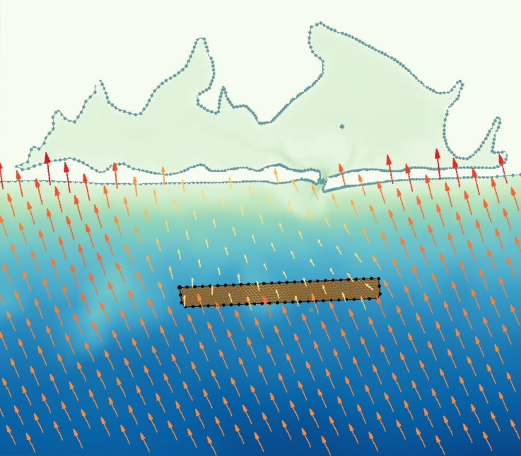
Example of a rubble mound in CMS-Wave

Rubble mounds in CMS-Wave simulations work a little differently than CMS-Flow. CMS-Wave doesn't have a specific rubble mound coverage like CMS-Flow does. Instead, rubble mounds are defined on a CMS-Wave structures coverage. This behaves somewhat similarly to materials coverages that you may be familiar with in other SMS models. Double-click the polygon representing the rubble mound to bring up the Assign Structure dialog. Then you'll add a structure with the green plus sign, select "Rubble-mound" from the structures dropdown, and then whether or not you want to modify the rubble mound by elevation. If you'd like, you have the option of customizing the color and texture SMS will use to fill your polygon structure to something that best suits your project.

CMS-Flow and CMS-Wave each require their own simulations, but you have the option to couple them using inline steering. This is a great option if you're building a comprehensive coastal model.

Head over to SMS and try out adding rubble mounds to your CMS project today!

Blog tags: 

Generating a 3D Grid from Raster Data

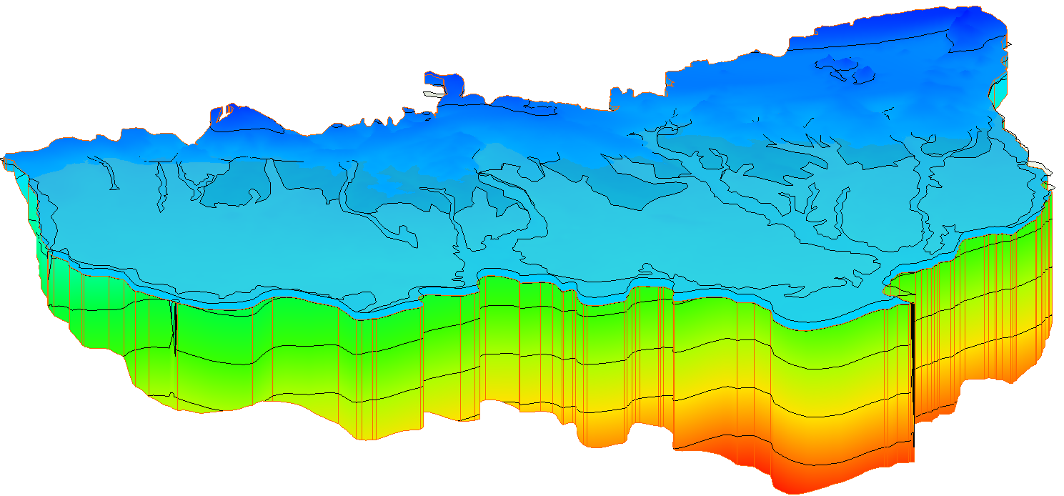
Have you heard about the 3D UGrid from Rasters tool that’s new to the Groundwater Modeling System (GMS)? Previous versions of GMS required you to build a raster catalog and then use the “Horizons to Solids” command in order to generate a 3D unstructured grid (UGrid) when modeling stratigraphy. The 3D UGrid from Rasters tool, which is in GMS’s toolbox under the “Unstructured Grids” folder, streamlines this process by allowing the two previously separate processes to be set up in the same place and executed simultaneously.

Example of a 3D UGrid generated from rasters

The base components for creating a UGrid with the 3D UGrid from Rasters tool are a 2D UGrid and multiple rasters. The rasters are then added to a table and assigned a horizon number. The term “horizon” refers to the top of each stratigraphic unit that will be represented in a corresponding solid, HUF unit, or 3D mesh layer. Horizons are ordered from the bottom up. For each raster you can choose to fill or clip the layer. Choosing “fill” tells GMS to use the raster to create a UGrid layer. Choosing “clip” tells GMS that any lower surfaces should truncate at that layer. You also have the option of creating sublayers between any rasters that have the “fill” option turned on. You can then set the relative size of each of the sublayers so that they are all proportional, or of differing sizes.

After setting all of the parameters for your UGrid in the rasters table, you then need to set a target location so that GMS knows to calculate elevations at the UGrid cell tops and bottoms or at the points. Lastly, you’ll need to define the minimum thickness that every layer must have, and choose a name for your new UGrid.

If you want more details about how the 3D UGrid from Rasters tool works, you can check out this page of our wiki. You can also look at the newest version of the Horizons with Rasters tutorial.

Head over to GMS, and use this new tool to simplify the stratigraphy modeling process.

Blog tags: 

Deciding between SRH-2D 2D Bridges and 3D Bridges

In the Surface-water Modeling System, you have the option of adding either a 2D or a 3D bridge to your SRH-2D model. But what are the differences between 2D and 3D bridges, and how can you know which one is the best fit for your SMS project? There are pros and cons to each, so we will briefly explore each option, and hopefully by the end you’ll have a better idea of what works best for you.

Starting in SMS 13.3, the 3D Bridge component that was used in previous versions was retired in favor of 3D Structures. 3D Structures can be used to build 3D bridges as well as culverts, and can also be used to calculate overtopping, an option that wasn’t available with 3D Bridges.

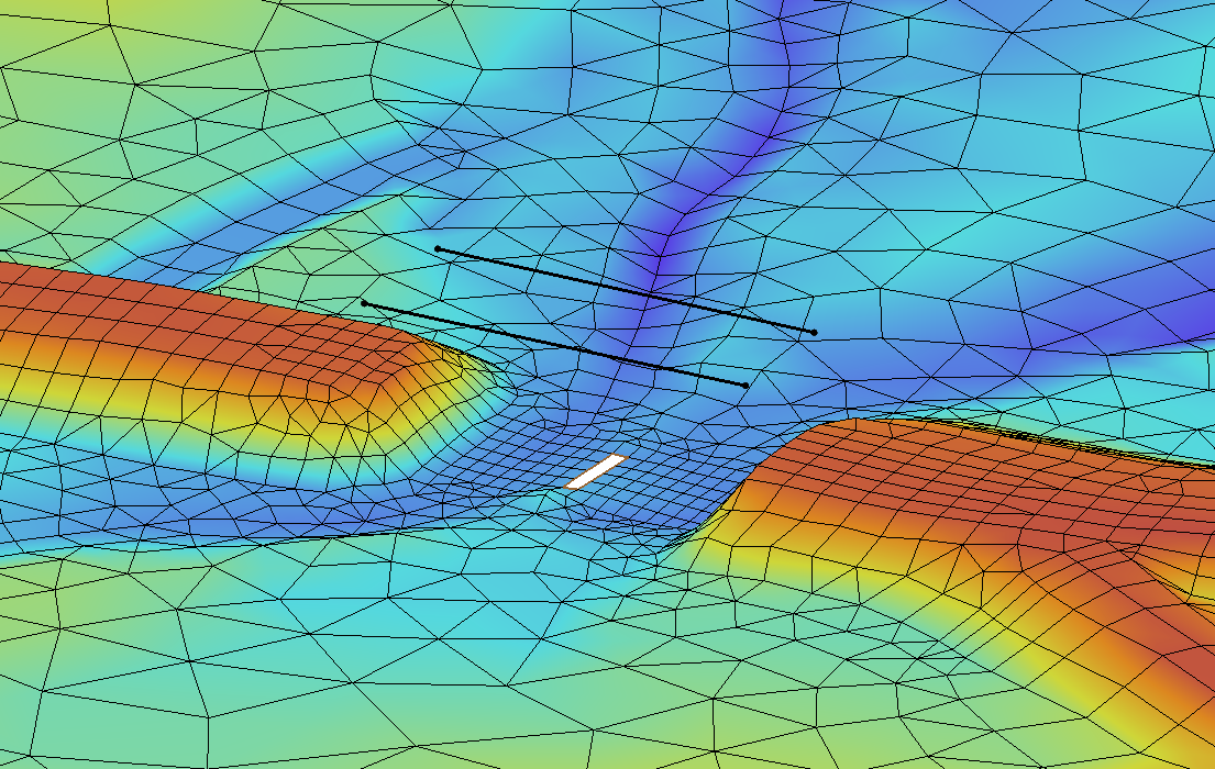
SRH-2D 2D bridge example

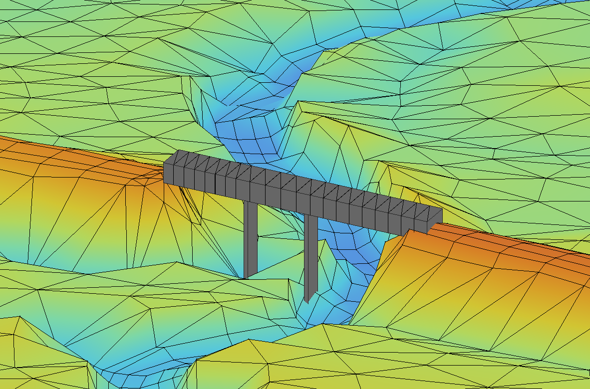
For 2D bridges, you have many options to help you customize your bridge, such as setting the bridge width, type and number of piers, abutments, etc.. (For the full list, go to this page of our wiki). All of the options that exist for 2D bridges are also available when building a 3D bridge. Using the 3D structures coverage to build your bridge allows for even more customization, including being able to shape the bridge ceiling so there is variation rather than being a constant along the full length.You can also use the 3D structures dialog to add a UGrid to the Project Explorer so that you can see what the bridge will look like with the mesh. The 3D structures coverage dialogue is able to generate a mesh footprint for your bridge, which automatically includes voids in the mesh for your piers so you don’t have to create them manually.

SRH-2D 3D bridge example

If you have questions about the specifics of building a 3D bridge, check out the new 3D Structures tutorials, or our wiki page on 3D Structures to get a more thorough introduction.

Building a 3D bridge into your project is an excellent option when you want to go the extra mile with the visual representation of the bridge. Although the idea of using a 3D bridge for everything may sound great because of the extra visualization options, a 3D bridge isn’t going to be necessary, or even practical, for every project. SMS’s calculations will turn out the same regardless of which bridge type you pick. 2D bridges are often a better choice if you’re looking for just a quick representation for your bridge, or if you’re modeling multiple bridges at the same time. Having multiple 3D bridges can slow down the processing speed in a way that having multiple of their 2D counterparts wouldn’t.

Head over to SMS and try out the 2D and 3D bridge building tools in 13.3 today!

Blog tags: 

Understanding SRH-2D's Monitor Coverage

Being able to determine hydraulic parameters at specific locations in the model domain is a handy, and sometimes even necessary, tool for any SRH-2D model. That is why there is a specific coverage in the Surface-water Modeling System (SMS) where you can create monitor objects that will collect the information you need during the simulation run. This blog post will cover some information that you may find useful when trying to make the most out of your monitor coverage.

SRH-2D outputs monitor data at a fixed interval of every 100 time steps. This is important to keep in mind if you’re looking to collect a certain amount of data from your monitor points or lines. You may need to adjust the size of the time steps depending on what kind of output you need.

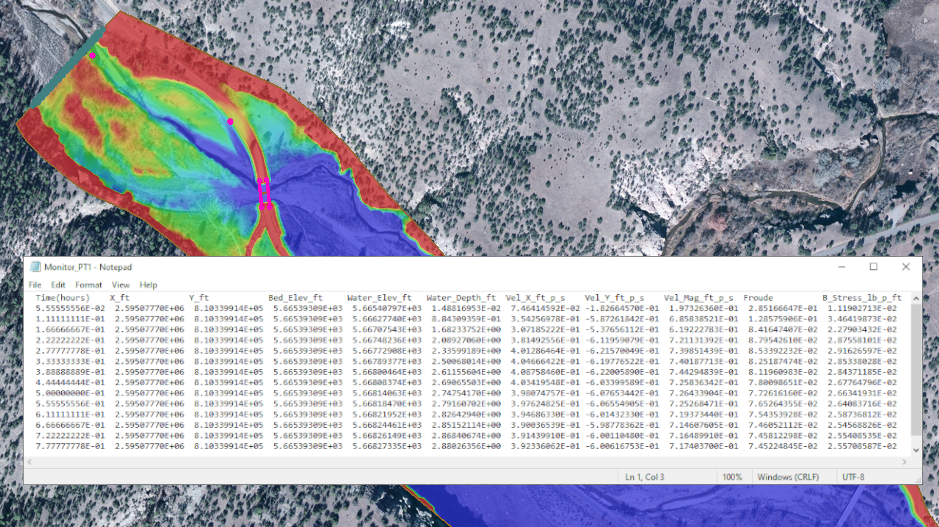
SRH-2D monitor points output file
Monitor Points

When creating monitor points on the SRH-2D monitor coverage, it is recommended that you create at least three monitor points: one near each end of the model domain, and one in the middle. During the simulation run, SRH-2D collects data at the points about a number of things, including but not limited to: the position in the X and Y direction, bed elevation, water elevation, and water depth.

Monitor Lines

Monitor lines can help you verify the continuity and model stability of your SRH-2D simulation. SRH-2D uses monitor lines to calculate the total flow and average water surface elevation along the arc. Monitor lines work best when they cross a river rather than running parallel. Lines with too many curves can cause difficulties in snapping to the mesh properly. Monitor lines can be placed anywhere along a river, but we recommend that one be created near the inflow and outflow boundaries. Remember to use monitor lines judiciously. Too many monitor lines can bog down your simulation, or even keep it from converging properly.

Monitor Output Files

Monitor output files are automatically exported to the location of the project files using this directory format: \[Project_Name]_models\SRH-2D\[Simulation_Name]\Output_Misc. The Output_Misc folder contains a DAT file for each of the monitor features using the *[Simulation_Name]_LNn.dat naming convention for lines, and *[Simulation_Name]_PTn.dat for points. These files contain all the data for each individual point or line, and can be opened in your prefered text editor application.

SRH-2D Solution Plots

We covered how SRH-2D solution and monitor plots work in a blog post a while back. If you’re interested in learning more about solution and monitor plots and how to use them, follow this link to our website.

Head over to SMS and try out the monitor coverage with your SRH-2D model today!

Blog tags: 

Introducing HydroGeoSphere with GMS

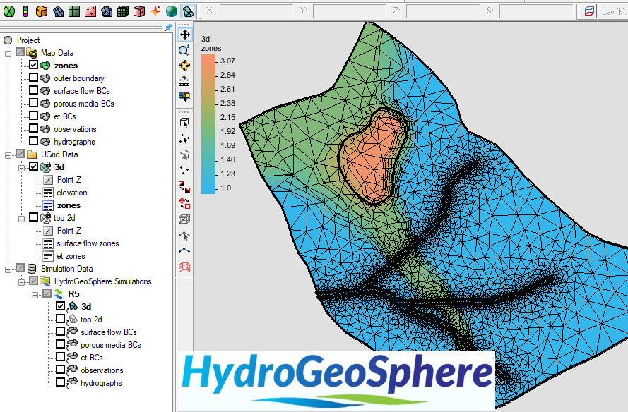
The Ground-water Modeling System (GMS) 10.8 beta includes a model interface that is brand new to the software. HydroGeoSphere (HGS) is a unique three-dimensional control-volume finite element simulator developed by Aquanty that is meant to be able to handle all parts of the terrestrial water cycle. It uses a globally-implicit approach to simultaneously solve the 2D diffusive-wave equation for overland/surface water flow and the 3D form of Richards’ equation for variably saturated groundwater flow. This is different from the many other models that simulate only a portion of the hydrologic cycle. HGS includes components for precipitation, evaporation, overland flow, infiltration, recharge, and more. HGS can simulate both surface and subsurface water flow simultaneously for each time step.

In GMS, the base components for an HGS model include: an unstructured (UGrid), HGS coverages, and an HGS simulation. GMS allows multiple HGS simulations to exist in a single GMS project. A 3D UGrid of the project area is required before building an HGS simulation. There can also be multiple UGrids in one project, although only one UGrid can be assigned to each simulation.

The coverages specific to HGS are boundary conditions, observations, and hydrographs. GMS uses feature objects to define the boundary conditions on an HGS boundary conditions coverage. This includes points, arcs, and polygons. The observations coverage allows you to set observation points that will collect time series information during the simulation run. The hydrograph coverage records hydrograph data during the simulation run.

HGS defines materials with domains and zones. The domain contains information about the type of material. The domain is then assigned a zone number, which is then assigned to a polygon. Multiple domains can be assigned to the same zone.

HGS with GMS

There’s a lot more to HydroGeoSphere than we can cover in one blog post. If you’d like to learn more about HGS, Aquanty has numerous resources on their website. You can look at the HGS Theory Manual or the HGS Reference Manual. They regularly post webinars on their blog and on their LinkedIn. You can also find videos about how to use HydroGeoSphere as well as presentations that have been made by Aquanty’s staff on their YouTube page. We also have our own HGS tutorials that can walk you through the steps of building an HGS model.

We hope you’re excited about the addition of HydroGeoSphere into GMS 10.8, because we certainly are! Download GMS 10.8 to try out HGS today!

Blog tags: 

Defining Elevation and Storage Capacity of Detention Basins

Did you know that the Watershed Modeling System (WMS) has a calculator that can define the relationship between the elevation and storage capacity of a detention basin? This is a useful tool for any WMS project with detention basins. The detention basins calculator is a simple tool that can quickly get the storage calculations you need for your model.

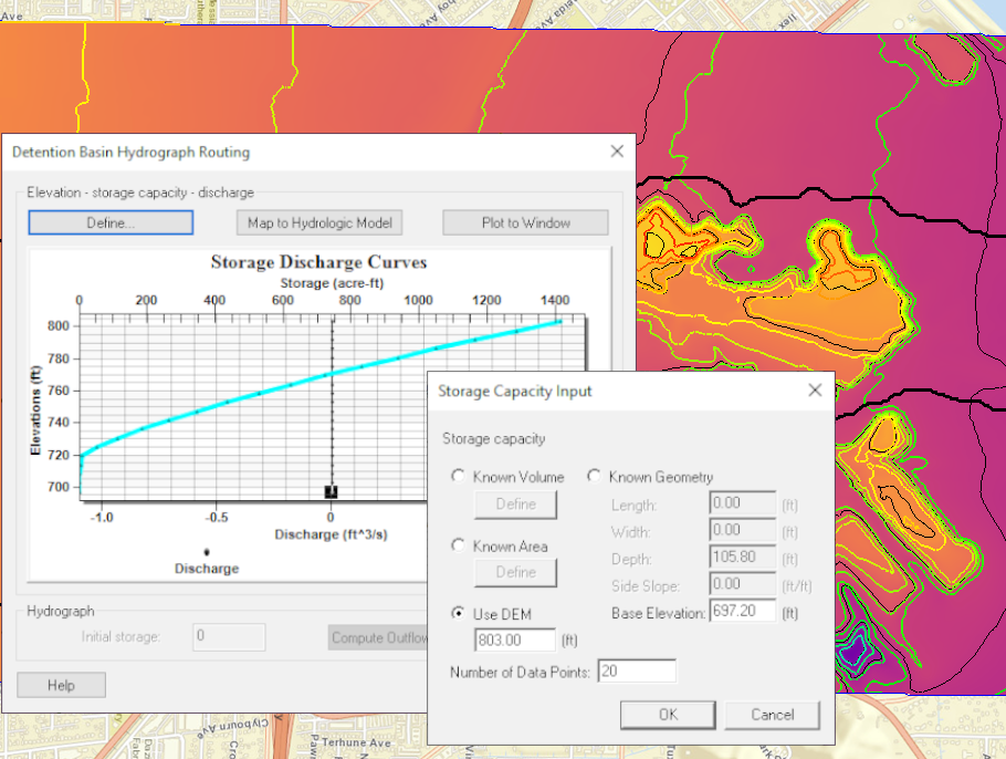
WMS uses the Hydraulic Toolbox to perform these calculations for the detention basin calculator. To open the detention basin calculator, first you need to make the Hydrologic Modeling Module active and select an outlet. Detention basins… is one of the options under the Calculator menu. After selecting Detention basins… a dialog named Detention Basin Hydrograph Routing will appear. Clicking the Define… button opens the Storage Capacity Input dialog, which is where you can enter the data that is needed for the calculations.

Basin Calculator in WMS

There are four data input options you can use to calculate storage capacity in the Storage Capacity Input dialog. Only one of the four input options is needed in order to perform the calculations. Which one you use will depend on what data is readily available for your model.

It is important to note that regardless of what measurement the general display projection is set to, the detention basin calculator will measure the elevation in feet and the storage volume in acres per foot.

After you exit the Storage Capacity Input dialog, a plot will be automatically generated in the Detention Basin hydrograph Routing dialog. This plot displays the relationship between the elevation and the amount of storage, as well as discharge if there is any. This plot functions the same way as any other plot window in WMS. You can learn more about plot windows by following this link to our wiki.

Head over to WMS to check out the detention basin calculator and see how you can use it to calculate the storage versus elevation for your detention basins today!

Blog tags: 

Handling Depth vs. Elevation

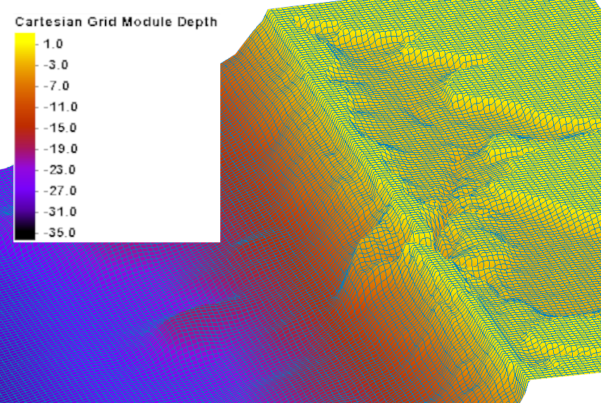
When creating a surface-water model, your model will make use of bathymetry data as either elevation or depth. Knowing how the Surface-water Modeling System (SMS) represents depth versus elevation is vital when it comes to creating, running, and understanding a model. SMS uses several different numerical models, and some models require that depth be negative and elevations be positive, while other models require the opposite.

It can become confusing when trying to remember what is needed for each model, which is why the decision was made to standardize how SMS treats elevation and depth across all models. SMS treats all depth values as negative and all elevation values as positive. That way you don’t have to remember how data needs to be entered for each model. If depth data is entered with positive values, SMS will read the data as part of the land elevations, which will produce incorrect calculations.

Depth/elevation shown on a grid

Some of the most used models where you may see that the elevation values have been changed to fit SMS’s conventions after importing are CMS-FLOW, CMS Wave, and CGWAVE. If you’re not sure whether or not the imported elevation data has been changed and would like to check, then this is a great time to make use of the Mesh module’s find function. Under both the Nodes menu and the Elements menu you’ll see a Find… option listed. You can use this to quickly locate a specific node or element inside of SMS to compare the elevation data with the model’s files outside of SMS.

If SMS has changed the values of the elevation data to account for the required negative depth value, there is no need to be concerned about how this will affect the end result for your model. SMS automatically adjusts the data to match the convention of the model when the project information is exported to the model executable.

Take this information and head over to SMS, more confident that your project’s elevation data will be handled correctly.

Blog tags: 

Troubleshooting MODFLOW in GMS

When constructing a MODFLOW model in GMS, there is always the possibility that you will get an error when trying to run your model. While there are a number of things that could be keeping your model from running without an error, here are some tips to help you figure out what may be going wrong.

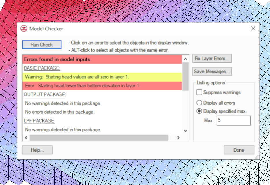
Example of the MODFLOW Model Checker

Before running MODFLOW, make use of the Model Checker. The Model Checker will analyze all the current input data for any obvious errors or potential problems, which could save you from having to hunt down individual input errors. The Model Checker gives you a few options for sorting and displaying errors. The Model Checker is a useful tool for a basic check of the inputs, however the Model Checker coming up clean doesn’t necessarily guarantee that the solution is correct.

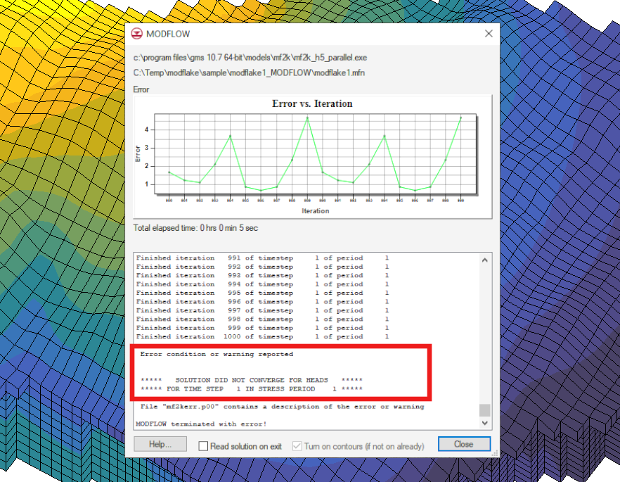
Example of the MODFLOW Model Checker The next thing to look at in your MODFLOW model when you’re trying to figure out what the issue may be is the command line output from the MODFLOW model wrapper dialog. When the model does not converge, an error message should appear in the command line output. This message will help you know where to start resolving the issue.

Another place to look when you’ve encountered an error is the MODFLOW output file (*.out) in the solution files in the Project Explorer. You can use this text file to check for any missing or incorrect values.

Now that we've covered some ways to check your MODFLOW model for errors, here is a common issues that may be what is keeping your MODFLOW model from converging properly:

  • An unbalanced flow budget. This can happen if the inflow is greater than the outflow, which causes extreme flooding, or if the outflow is greater than the inflow, which would cause all cells to go dry.
  • All grid cells in the model are assigned a specified head boundary condition. This leaves nothing for MODFLOW to compute, causing the model to terminate with an error.
  • Improper initial conditions or boundary conditions.
  • You have a highly sensitive model. Highly sensitive areas might keep MODFLOW from converging due to the speed at which flow can be affected.
  • Elevation and layer values have been incorrectly defined or have inaccuracies.

Additional information can be found in the Frequently Asked Questions section of the MODFLOW user manual under the question "My model hasn’t converged. What can I do?"

Use these tips to help your MODFLOW model run smoothly in GMS.

Note this is an update to a previouisly published blog post.

Blog tags: 

Pages