GMS

New MODFLOW-USG 3D Dataset to Array

By aquaveo on March 26, 2024

While most groundwater projects typically only need a 2D dataset to define arrays, 3D datasets are becoming more available. There’s a new feature in the Ground-water Modeling System (GMS) version 10.8 for MODFLOW-USG and MODFLOW-USG Transport models. MODFLOW-USG and MODFLOW-USG Transport are MODFLOW models that were designed specifically to be used with unstructured grids, or UGrids. The Recharge (RCH), Evapotranspiration (EVT), and EvapoTranspiration Segments (ETS) packages in MODFLOW-USG now have the option to use a 3D dataset to define the input arrays. Previous versions of GMS only had the option to use a 2D dataset with a matching 2D structured grid.

Example of the 3D Dataset to Array option

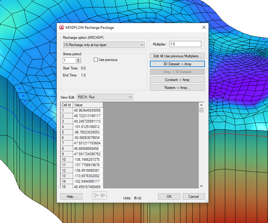
You can find the 3D Dataset → Array button in the properties dialog of the Recharge (RCH), Evapotranspiration (EVT), or EvapoTranspiration Segments (ETS) package. In order to use the 3D Dataset → Array button, the 3D dataset in the MODFLOW-USG model has to have the same number of rows and columns as the 3D grid. If the rows and columns don’t match the 3D grid, then the button will be grayed out and you won’t be able to use it.

Clicking the 3D Dataset → Array button will bring up a Select Dataset dialog with a list of all the datasets associated with the current 3D grid. You can then select the relevant dataset to assign values to the MODFLOW-USG package. 3D datasets are often created using the 3D Scatter Point tool, which can help you interpolate rainfall data to the cells on your grid. If you are using a transient dataset, then the dataset values will be interpolated linearly to each stress period when they are copied to the array. You can learn more about using the 3D Scatter Point tool on this page of our wiki.

Now head over to GMS 10.8 and try using the new 3D Dataset → Array button in your MODFLOW-USG or MODFLOW-USG Transport project today!

Blog tags:

GMS

Understanding Pass Through Cells

By aquaveo on March 5, 2024

Starting with version 10.8, the Groundwater Modeling System (GMS) has the ability to handle pass through cells in MODFLOW-USG and MODFLOW-USG Transport projects. What are pass through cells? If you have a 3D UGrid with multiple layers, you can have middle layers with pinchouts or other features that cause that middle layer to not extend through the entire range of the other layers. For example, if you have a three-layer unstructured grid with a pinchout in layer two, then you will have an area where the cells of layer one and layer three are supposed to meet. This area where a middle layer is missing for some of the cells is where pass-through cells are needed.

In actuality, there is a thin cell between the layers. Because of this, in areas where a middle layer is missing a barrier would be formed when running MODFLOW-USG. If you don’t want a barrier in that area, then you will need to add a pass through cell to allow water to flow through the area. This means you need to have the Ibound be greater than zero or the water will not be able to pass through the middle layer and create a “no-flow zone.”

By switching between layers you can see which layers have a thickness of zero and which do not. To inactivate the cells with a thickness do the following:

Open the MODFLOW Global/Basic Package dialog.
Select the Set Pass Through… button.
A message will appear explaining parameters used to determine pass through cells.
In the Pass Through Thickness dialog, set the maximum cell thickness.

After assigning the maximum cell thickness, cells that are below that thickness will be designated as pass through cells. The pass through cells will have an inactive IBOUND and will be ignored when making vertical connections in the DISU package.

Note that setting pass through cells requires a stacked grid.

Now that you know about pass through cells, make use of them in your MODFLOW-USG and MODFLOW-USG Transport projects in GMS today!

Blog tags:

GMS

Generating a 3D Grid from Raster Data

By aquaveo on February 13, 2024

Have you heard about the 3D UGrid from Rasters tool that’s new to the Groundwater Modeling System (GMS)? Previous versions of GMS required you to build a raster catalog and then use the “Horizons to Solids” command in order to generate a 3D unstructured grid (UGrid) when modeling stratigraphy. The 3D UGrid from Rasters tool, which is in GMS’s toolbox under the “Unstructured Grids” folder, streamlines this process by allowing the two previously separate processes to be set up in the same place and executed simultaneously.

Example of a 3D UGrid generated from rasters

The base components for creating a UGrid with the 3D UGrid from Rasters tool are a 2D UGrid and multiple rasters. The rasters are then added to a table and assigned a horizon number. The term “horizon” refers to the top of each stratigraphic unit that will be represented in a corresponding solid, HUF unit, or 3D mesh layer. Horizons are ordered from the bottom up. For each raster you can choose to fill or clip the layer. Choosing “fill” tells GMS to use the raster to create a UGrid layer. Choosing “clip” tells GMS that any lower surfaces should truncate at that layer. You also have the option of creating sublayers between any rasters that have the “fill” option turned on. You can then set the relative size of each of the sublayers so that they are all proportional, or of differing sizes.

After setting all of the parameters for your UGrid in the rasters table, you then need to set a target location so that GMS knows to calculate elevations at the UGrid cell tops and bottoms or at the points. Lastly, you’ll need to define the minimum thickness that every layer must have, and choose a name for your new UGrid.

If you want more details about how the 3D UGrid from Rasters tool works, you can check out this page of our wiki. You can also look at the newest version of the Horizons with Rasters tutorial.

Head over to GMS, and use this new tool to simplify the stratigraphy modeling process.

Blog tags:

GMS

Introducing HydroGeoSphere with GMS

By aquaveo on January 23, 2024

The Ground-water Modeling System (GMS) 10.8 beta includes a model interface that is brand new to the software. HydroGeoSphere (HGS) is a unique three-dimensional control-volume finite element simulator developed by Aquanty that is meant to be able to handle all parts of the terrestrial water cycle. It uses a globally-implicit approach to simultaneously solve the 2D diffusive-wave equation for overland/surface water flow and the 3D form of Richards’ equation for variably saturated groundwater flow. This is different from the many other models that simulate only a portion of the hydrologic cycle. HGS includes components for precipitation, evaporation, overland flow, infiltration, recharge, and more. HGS can simulate both surface and subsurface water flow simultaneously for each time step.

In GMS, the base components for an HGS model include: an unstructured (UGrid), HGS coverages, and an HGS simulation. GMS allows multiple HGS simulations to exist in a single GMS project. A 3D UGrid of the project area is required before building an HGS simulation. There can also be multiple UGrids in one project, although only one UGrid can be assigned to each simulation.

The coverages specific to HGS are boundary conditions, observations, and hydrographs. GMS uses feature objects to define the boundary conditions on an HGS boundary conditions coverage. This includes points, arcs, and polygons. The observations coverage allows you to set observation points that will collect time series information during the simulation run. The hydrograph coverage records hydrograph data during the simulation run.

HGS defines materials with domains and zones. The domain contains information about the type of material. The domain is then assigned a zone number, which is then assigned to a polygon. Multiple domains can be assigned to the same zone.

There’s a lot more to HydroGeoSphere than we can cover in one blog post. If you’d like to learn more about HGS, Aquanty has numerous resources on their website. You can look at the HGS Theory Manual or the HGS Reference Manual. They regularly post webinars on their blog and on their LinkedIn. You can also find videos about how to use HydroGeoSphere as well as presentations that have been made by Aquanty’s staff on their YouTube page. We also have our own HGS tutorials that can walk you through the steps of building an HGS model.

We hope you’re excited about the addition of HydroGeoSphere into GMS 10.8, because we certainly are! Download GMS 10.8 to try out HGS today!

Blog tags:

GMS